Zeners behave like...
This page was created based (mostly) upon data downloaded directly from an oscilloscope with the following sample regime: 100 kSa/s with a 1.2 MSa depth @ 500 mV/div. Thus $\epsilon = 15.6 \text{ mV}, \tau = 10 \mu \text{s}$. We used our Zener Variator to vary the reverse current $(I_R)$ for these experiments, which has a floating noise floor (1000 mm flying leads) of approximately 304 mVpp. The diodes used were 51V, 24V and 10V through hole Zeners.
The signal
Our results for various $I_R$, featuring oscilloscope screen shots and Gnuplots of downloaded scope memory values:-
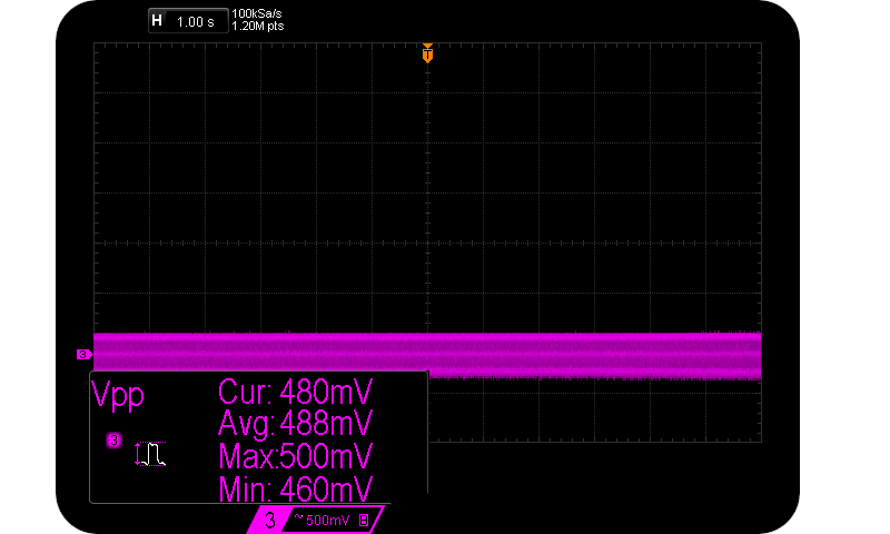
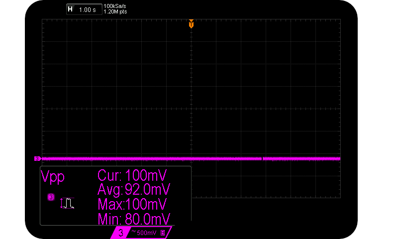
51V Zener diode @ 5 uA $I_R$.
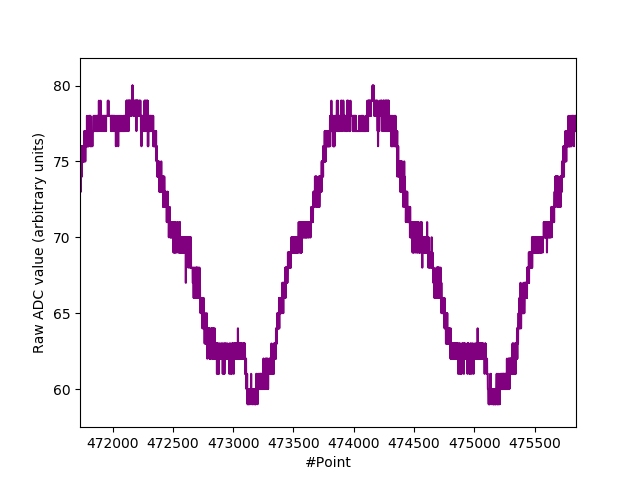
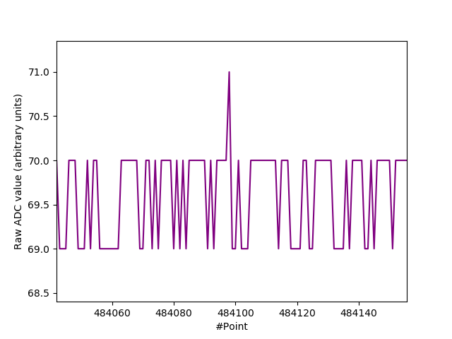
51V Zener diode @ 5 uA $I_R$. (Scope download).
Very little of interest to see above. It’s mainly our 50Hz mains hum as $I_R$ is so low and our leads so long. But quantization noise of same is evident.
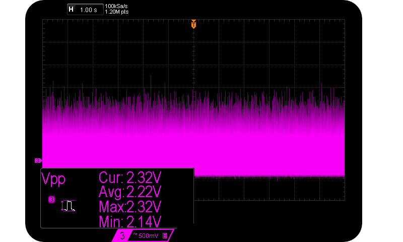
51V Zener diode @ 50 uA $I_R$.
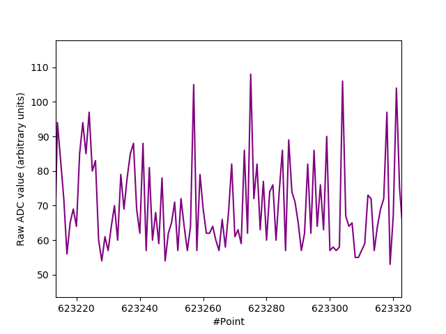
51V Zener diode @ 50 uA $I_R$. (Scope download).
Proper avalanche behaviour is evident above. One simple way to tell is that one side of the plot is spiky, whilst the other side is much smoother. This is characteristic of log-normal distributions. Notice the relatively massive Avalanche signal $(V_{pp} = 2.22 \text{V for } I_R = 50 \mu \text{A})$. It is indicative of $V_{pp} \propto V_Z$. The following figure highlights the shape of the distribution more clearly:-
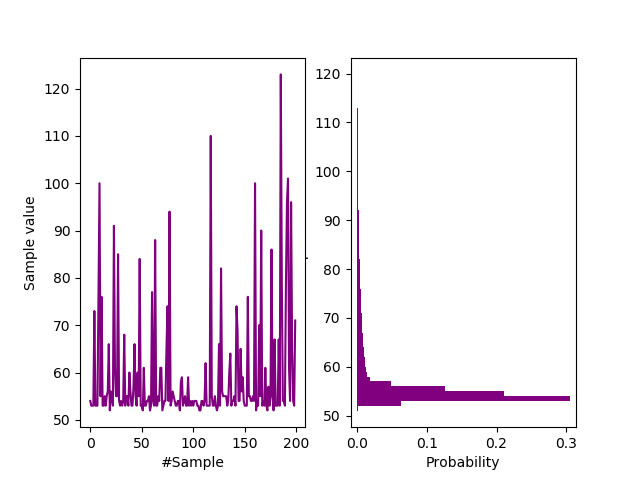
Waveform and (log normal) probability mass function for a 51V Zener diode in Avalanche.
If autocorrelation was sufficiently small $(R \le 10^{-3})$, we could immediately quantify $H_{\infty} = - \log_2 (0.3) = 1.7$ bits/sample (scope download). But we haven’t checked in this particular case. Notice though the extreme log-normal shape, characteristic of well proper Avalanche behaviour.
We now increase $I_R$ to $100 \mu \text{A, } 150 \mu \text{A, } 300 \mu \text{A & } 500 \mu \text{A}$:-
51V Zener diode @ 100 uA $I_R$.
51V Zener diode @ 150 uA $I_R$.
There are only a few rare peaks at $I_R = 300 \mu \text{A})$:-
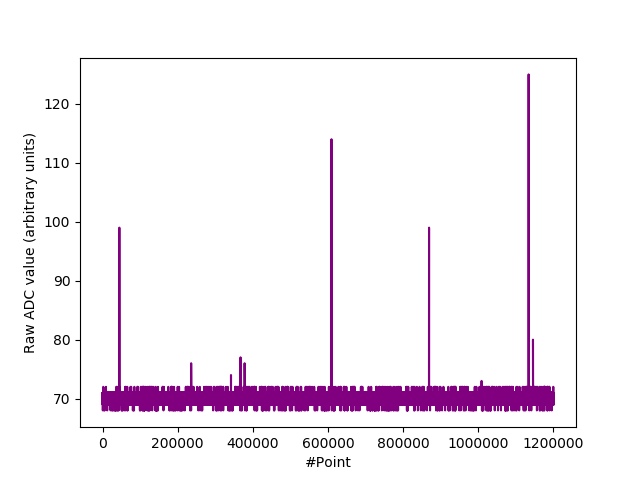
51V Zener diode @ 300 uA $I_R$. (Scope download).
And no peaks at $I_R = 500 \mu \text{A}$. The bulk of the signal is now just quantization noise of a few bits:-
51V Zener diode @ 500 uA $I_R$.
51V Zener diode @ 500 uA $I_R$. (Scope download).
The entropy
Entropy is after all, our business here. Not simply humongous $V_{pp}$ values. And we see below that the usable entropy from a Zener diode’s Avalanche signal is not entirely proportional to it’s peak to peak magnitude. It’s a much more complicated relationship.
We looked at three diodes with $ 5 \mu \text{A} < I_R < 500 \mu \text{A} $ with differing $V_Z$ using the Zener Variator and oscilloscope. We then downloaded the 1.2 million raw oscilloscope samples (8 bit depth) and compressed them using the LZMA compression algorithm. We can estimate the Shannon entropy $(H_S)$ of the samples, and thus the generating rate as bits per second.
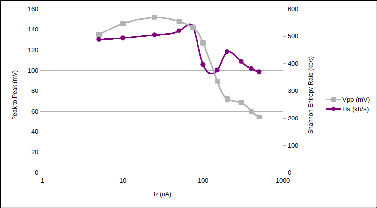
51V Zener noise and entropy rate vs $I_R$.
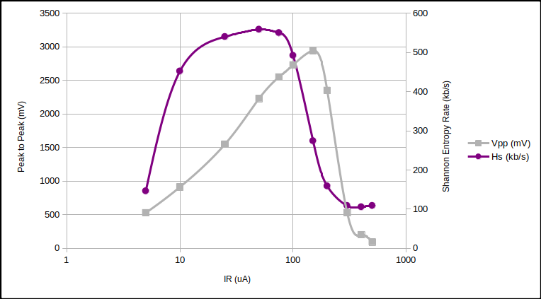
24V Zener noise and entropy rate vs $I_R$.
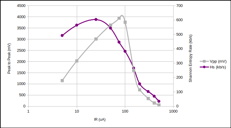
10V Zener noise and entropy rate vs $I_R$.
Combining the three above graphs and normalising $H_S$:-
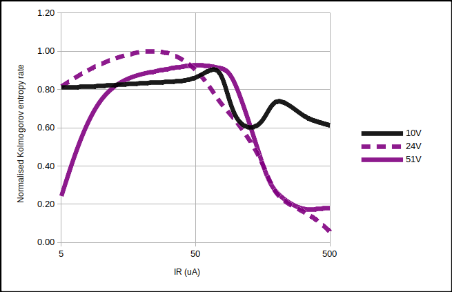
Normalised Kolmogorov entropy rates vs $I_R$.
The surprising point to note from the above curves is how similar the entropy rate is between different diodes at $I_R \approx 50 \mu \text{A}$. Quantisation error is responsible for a large proportion of that rate. But…
The conclusion
One might initially assume that more $V_{Z}$ implies more $H_{S}$. Common sense, and of course size matters. Yet if we look at these three stylised Zener signals, that’s not the case due to a quirk of the Avalanche effect:-
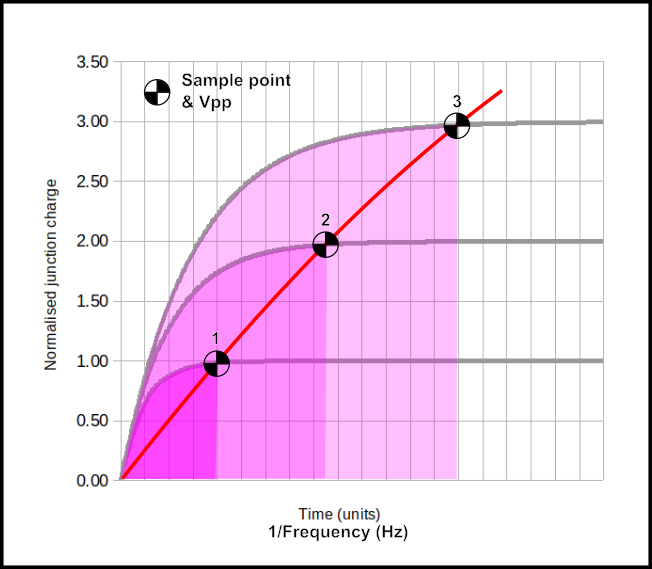
Normalised magnitude and duration of 3 Avalanche pulses differing in PN junction charge (exaggerated).
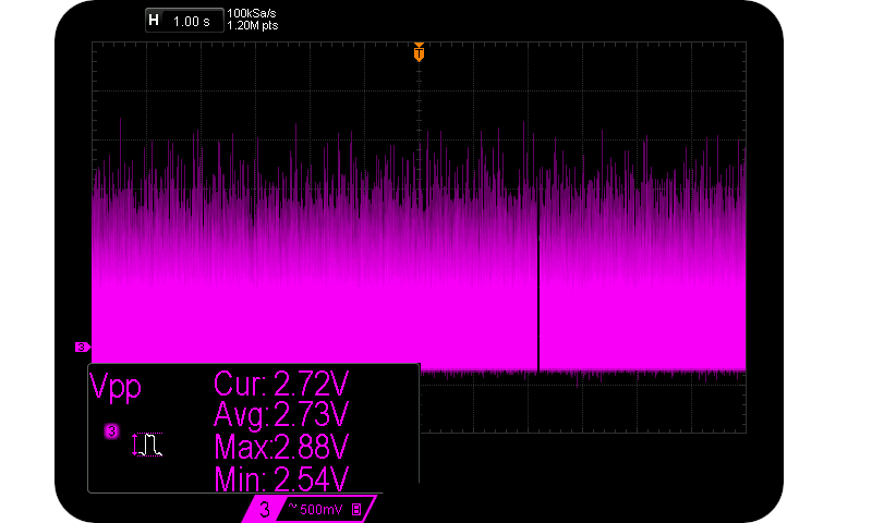
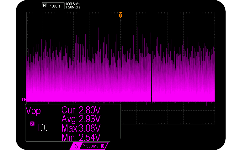
Assume that we are interested in maximising $V{pp}$ and thus $H_{S}$, so we look to higher and higher reverse voltages. We sample at the marked sample points (about 95% $V{pp}$). However the exponential charge shape remains a fairly similar geometry, just larger and wider. As the normalised charge ratio increases (and so does $V{pp}$), the time between potential sample points also increases. I.e. the frequency of large pulses decreases. The approximate $Vpp \propto \frac{1}{f_{V_{pp}}}$ relationship is verified in the following two scope captures caused by $55 \mu \text{A} < I_R < 125 \mu \text{A}$:-
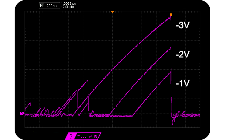
Actual magnitude and duration of 3 Avalanche pulses differing in Vpp.
Rare 3 Vpp & common 1 Vpp Avalanche pulses.
Notice how sparse other peaks are for the case of $V_{pp} = 3 V$. And so that’s how $H_S$ isn’t as large as one might expect. Size in this case does not matter as far as entropy is concerned.
Which explains the “Normalised Kolmogorov entropy rates vs IZ” figure above. A plus side though is that high voltage Zeners are not required to obtain decent entropy rates from them. It’s not about getting the largest Avalanche signal that matters, but obtaining the most entropy from it.
The discussion
-
We might well expect $H_{\infty} \sim 1$ bits/sample from simple quantisation error given the large and (virtually) infinite resolution noise signal, and the relatively small oscilloscope sampling resolution (8 bits). But more on this elsewhere.
-
The quantum unit responsible for the ultimate resolution of the Avalanche noise is a single electron. It’s charge ($e$) is $1.60 \times 10^{-19}$ Coulombs.
-
Sampling at 100 kSa/s (which an Arduino can) and with $I_R = 50 \mu \text{A}$, we can calculate that $3.125 \times 10^9$ electrons are flowing through the Zener diode every $\frac{1}{100,000}$th of a second. $\pm 1e$ at the very minimum. That’s a resolution of 0.32 parts per billion. Or over 31 bits of resolution. Or a minimum discrete Avalanche current change to constant current (signal to noise) ratio of -190 dBV ($1 e$).
-
All the diodes vary, but with a loose correlation for Avalanche $V_{pp} \propto V_Z$, as shown below. That means that each device has to be treated individually and the entropy rate determined accordingly (which is also dependant on your $(\epsilon, \tau)$ sampling regime). Except for transistors as their reverse breakdown voltages do not range as widely as do Zener diodes'.
Some other examples of diodes’ and transistors’ $V_{pp}$ accumulated from us and across the internet:-
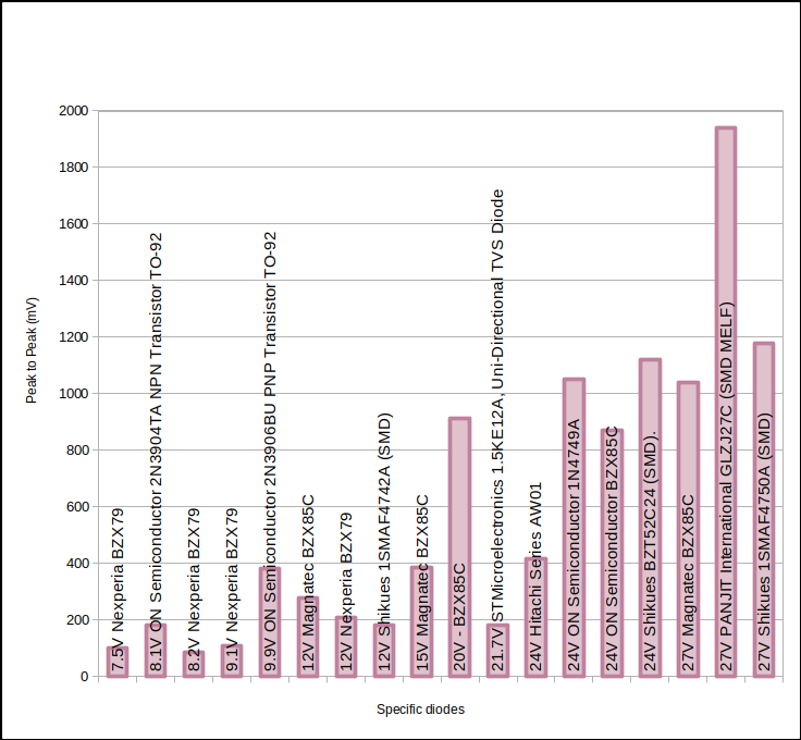
Avalanche Vpp for our other specific devices and packages.
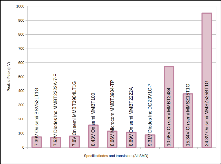
Avalanche Vpp for more other specific devices.
Above from https://betrusted.io/avalanche-noise
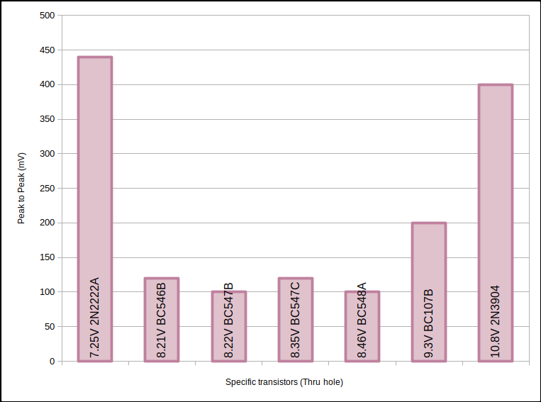
Avalanche Vpp for and more other specific transistors.
Above from http://holdenc.altervista.org/avalanche/