Entropy measurement
This page has been superseded with a more accurate entropy measurement technique here…
As this section deals with entropy ($H$), we thought that it might be useful to show you some of the purest kind. This is one of the team, Dom, demonstrating (very bad) entropy. Bad, bad, bad; he’s laid on a nice Hi-Fi speaker cover that he’s just pulled off:-
Dom. The purest kind of entropy.
Since the entropy sources on this site are to form the basis of TRNGs, there is Golden rule 3 that must be met, namely that $H_{in} > H_{out}$. Otherwise the device will simply be a PRNG with some unpredictable entropy bits thrown into the state. We’re interested in the pure stuff, but this then necessarily demands a measure of $H_{in}$. And therein lies the problem.
The crucial aspect is that we consider the raw .jpg file and not the opened/decoded raster image. Our JPEGs ~ 21.4 kB. Intuitively those files’ entropy cannot exceed the filesize. A typical rendered 640 * 480 pixel image creates a lossless PNG file of 284kB using maximum compression. This creates the false impression that the entropy may be in the 100s of kB. What actually happens is that the JPEG algorithm acts similarly to a PRNG seeded by xxx.jpg as $ G:\{0, 1\}^{|xxx.jpg|} \to \{0, 1\}^{|raster|} $, generating a 43 fold expansion in our case. Do not open the image!
It’s tempting to use the traditional Shannon [1] $H = -K\sum_{i} {p_i \log p_i}$ formula, but that would be wholly inappropriate in this case due to inherent correlations within the sample. The JPEGs’ probability distribution looks like the following, taken over 100 samples:-
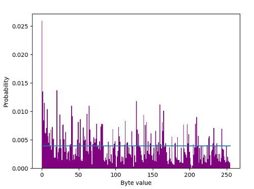
Byte value distribution in 100 JPEGs.
and the blue line is what it should be to be uniformly distributed with a $p = \frac{1}{256}$ or 0.0039. 0 occurs at twice the rate compared to the next nearest byte value. Arithmetic mean value of the bytes is 108.8, whereas it should be 127.5 if random. So not particularly random according to ent, but it returns (under an incorrect IID assumption) an entropy measurement of 7.66 bits per byte. Yet it’s perfectly random. Random $=$ uncertain. Random $\neq$ uniformly distributed. Reiterating, herein lies the problem. What we have is a massively correlated set of data which is entirely understandable as it’s JPEG encoded. You might characterise it as a correlated ergodic bit fixing source. The task is to measure the entropy of a JPEG file allowing for said correlation. The NIST tools that implement the entropy measurements of NIST Special Publication (SP) 800-90B, Recommendation for the Entropy Sources Used for Random Bit Generation are proven as unreliable or at least risky. Similarly, a min.entropy calculation is unsuitable for the reason that auto correlation makes obtaining a $p_{max}$ difficult. A $H_{\infty}$ defined simply by $-\log_2 (p_{max})$ of 5.27 bits per byte based on 0 being by far the most common is an initial very much upper bound estimate, but ignoring all correlations.
Fortunately, that document’s §6.3.4 The Compression Estimate offers a useful pointer. The compression estimate computes the entropy rate of a dataset, based on how much that dataset can be compressed and that you cannot losslessly compress anything below it’s entropy content. The estimator is based on the Maurer Universal Statistical test. The previous draft version of SP 800-90B (August 2012 Draft) also recommended the Burrows-Wheeler BZ2 compression algorithm as an entropy sanity check in §9.4.1. We can rewrite their compression test as $ |BZ2(S_i)| = H \lfloor \frac{N}{10} \rfloor + \Delta $, where $\Delta$ is an indicator of compressor inadequacy and overhead. We can now do much better than Burrows-Wheeler, and as the efficiency of the compression algorithm improves, $ \Delta \rightarrow 0 $ and thus compressive entropy measurement becomes a NIST sanctioned technique. It is of course also used in 90B (§5.1) for compression based IID determination. The scomp test within the TestU01 randomness test suite also uses compression, this time based on the Lempel-Ziv (LZMA) algorithm. And since the Lempel-Ziv algorithm consists of just 26 lines of pseudo code, there are much more efficient and advanced compressors.
Even without considering that the entropy is packaged in the binary format of the JPEG specification, autocorrelation is large. Especially within the first 50 bytes of each frame, reaching nearly 0.2. This can also be seen as a clear discontinuity between frames within the raw sample set:-
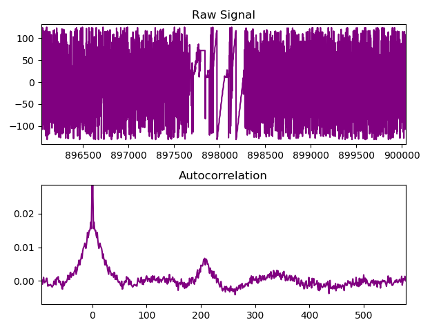
Autocorrelation analysis featuring JPEG boundary.
An alternative autocorrelation/IID test is our permuted compressions test, based on the 800-90B Compression Estimate and sanity check. However we use a combination of algorithms rather than just BZ2. The test is based on the principle that a permuted correlated file will not compress as well as the original correlated file For a 1 MB file of 50 concatenated frames, as expected, the IID test fails:-
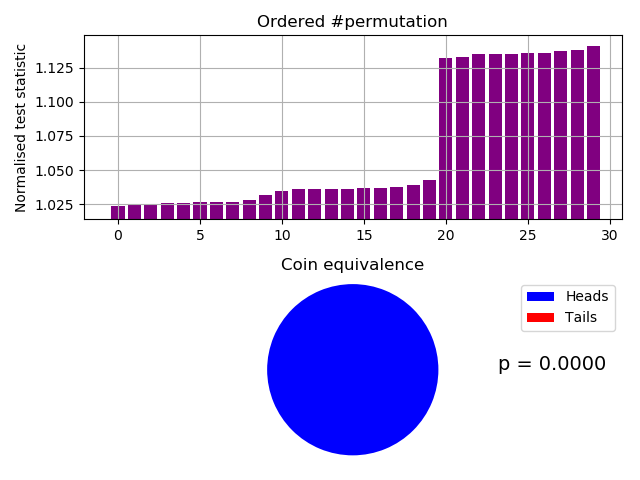
Badly failing custom permutation IID test.
There is also an alternative to the alternative, in the form of a conceptual entropy shmear measure. Strangely, the life sciences seem to use compression for entropy estimation much more than typical TRNG designers do. It’s used for example in protein folding assessments, fetal heart rate characterization and even music identification.
We constructed a data set from the Photonic Instrument comprising 100 concatenated JPEGs of overall size 2,120,003 bytes. Using paq8px from the Hutter Prize compression competition, our data set compressed to 1,310,191 bytes. This level of JPEG compression is achieved by partially decoding the image back to the DCT coefficients and recompressing them with a much better algorithm than the default Huffman coding. The cmix compressor (from the same competition) could not achieve a smaller compressed size as it does not incorporate JPEG models. Even recent asymmetric numeral system based compressors cannot achieve such a high degree of compression. $H$ was then calculated as 4.94 bits/byte across the JPEG data set. The fact that we can losslessly recompress the JPEGs to below the lossy $H_{\infty}$ value of 5.27 bits/byte demonstrates the level of correlation within the data set, and validates our methodology.
Compression algorithms have improved over time, and the following graph illustrates the decreasing records in the 12 year old Hutter competition:-
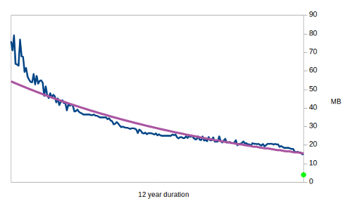
Compressed size of 100MB enwik8 test file.
Logically there must be an absolute lower bound to entropy of any given sequence as the Pigeonhole principle always applies. Otherwise we would not be able to differentiate one piece of information from the next. The fitted purple curve does seem to suggest that there is an asymptotic minimum compressible size for the competition’s 100MB enwik8 file. Perhaps it may go as low as 10MB. We thus divide 4.94 by a safety factor of 2, and again by 2 for ultra conservatism, uber security and just becoz’. Incidentally, the same conservative level of prediction would result in a compressed enwik8 file size of 3.82MB (the green dot on the compression graph). We therefore posit that the Photonic Instrument’s entropy rate is 1.235 bits per byte. Which to us looks like 1 bit per byte for simplicity’s sake. And 1 is something that Dom can understand. There are also benefits to this conservative entropy assessment in safely (and simply) accommodating temperature effects.
The mean size of JPEGs from the Photonic Instrument is 21.2kB. With $H_{\infty} = 1$ bit/byte, the instrument can safely generate approximately 212kb/s of entropy with it’s maximum frame rate of 10 frames/s. Or 26.5kB/s of IID bytes if we ignore processing time for randomness extraction.
This page has been superseded with a more accurate entropy measurement technique here…
References:-
[1] A Mathematical Theory of Communication, Claude E. Shannon, Bell Telephone System Technical Publications, 1948.