Shannon++
“An interesting question in all these contexts is to what degree these sequences can be ‘compressed’ without losing any information. This question was first posed by Shannon in a probabilistic context. He showed that the relevant quantity is the entropy or average information content h, which in the case of magnets coincides with the thermodynamic entropy of the spin degrees of freedom. Estimating the entropy is non-trivial in the presence of complex and long range correlations.” - Thomas Schürmann and Peter Grassberger.
Or why the Shannon entropy equation can’t be implemented in the general case 😞
The ubiquitous (notorious?) $ H = -K \sum_{i} p_i \log_{} p_i $ Shannon equation is commonly taken to determine the entropy of general sources. The problem is determining $i$ when the equation is implemented. Consider the most complex and autocorrelated source of entropy, natural languages:-
- nd, st, mm, gh digraphs often appear together, whilst u always follows q in the English language.
- “Prophet Muhammad (peace be upon him)” is considered a complete spoken phrase, with an autocorrelation lag of n = 35. And it contains mm.
- Llanfairpwllgwyngyllgogerychwyrndrobwllllantysiliogogogoch is a single Welsh village name. That’s 58 characters (51 “letters” since “ch” and “ll” are digraphs, and are treated as single letters in the Welsh language). n = 57 or 50, depending.
- ssi is an English trigraph to write the sound ʃ in words such as mission. n = 2.
- A play about Romeo and Juliet sees the words Romeo and Juliet appearing frequently, sometimes together and sometimes separately.
- And there is a full stop in English roughly every twenty words. n $\approx$ 89 based on a mean of 4.5 letters/word.
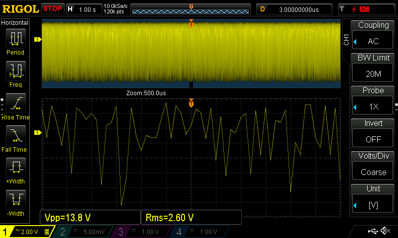
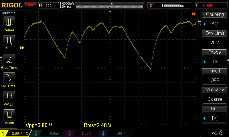
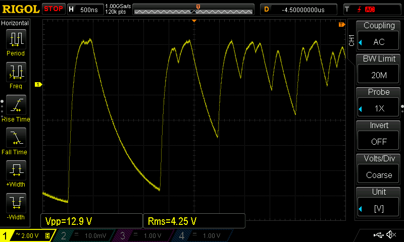
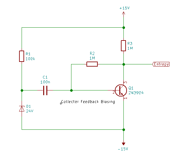
There are orthographic, syntactic and semantic issues that confound a simple enumeration of the domain of $i$. For a general unknown source, estimating the (min)entropy is far from trivial. Our TRNG situation is somewhat mitigated by the fact the natural language is much richer than analogue to digital converter readings of say chaotic laser intensity. Still, capacitative effects, experimental bias, too rapid sampling and dead/recovery times of various sensors can introduce aliasing and correlations spanning 1000’s samples. It’s just that the correlations are mathematically simpler, as in the following example of an over sampled Zener entropy source with nice smooth curves:-
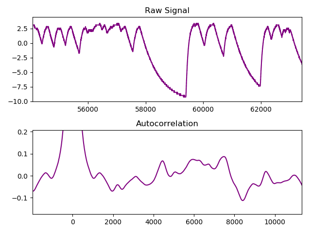
Obvious strong autocorrelation exceeding $\left| 0.1 \right|$.
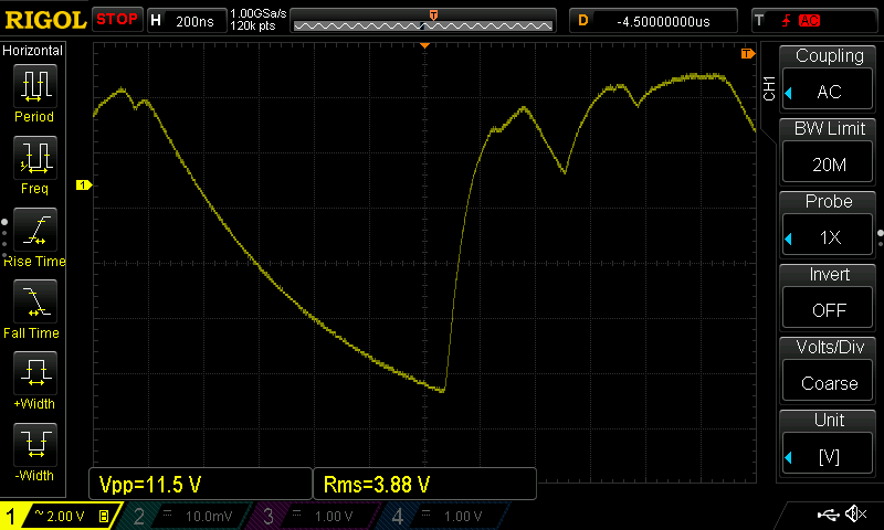
Still, the problem is intractable for any reasonable sampling circuit with limited size [Herrero-Collantes, Garcia-Escartin] . This particular waveform above (call it $ \pi:\{Y_1,\ldots,Y_t \}$) is governed by the normal capacitor charge curve: $ \pi \sim -C_1 \big(1 - e^{-\frac{t - t_a}{C_2}} \big) $ where the constants $ C_1, C_2 $ represent the signal voltage at the start of avalanche, and the time constant based on the resistance around the diode and it’s internal junction capacitance respectively. $t_a$ represents the temporal start of an individual electron cascade initiating the avalanche effect. Not a strict Markov sequence, but clearly algebraically correlated over many discrete samples. This data sample (1.2m-ascii-samples.zip) is available in the related files ↓.
To simply illustrate the entropy measurement for $\pi$, one might use a toy and (very) stylised multi-level thresholding scheme. As all of the waveform components are similar, a basic alphabet can be loosely established based on the threshold levels, like so:-
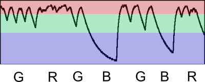
Stylised thresholding scheme for Zener signal $\pi$.
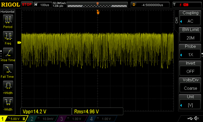
Multiple samples are therefore amalgamated into a [GRGBGBR] sequence. Algebraic correlation has effectively grouped the many discrete samples into far fewer ones, with a consequential reduction in entropy rate per real sample. Interesting factoid; the above data set represents a Shannon entropy rate of only 1.05 bits/sample as $\pi$ was (way) over sampled at 1 GSa/s to illustrate the point. This tuple of $(\epsilon, \tau)$ values is essentially equivalent to just one bit quantization jitter over an almost constant voltage.
The typical application of Shannon’s equation gives a much higher and entirely misleading entropy rate of 49.9 bits/sample by ignoring long range autocorrelations of the order > $\left| 0.1 \right|$. This is the problem with naively enumerating $i$, and is dangerous from a cryptographic security perspective. It’s also nonsensical as the sampling was performed with an 8 bit oscilloscope. This weirdness is in part also due to ASCII float to binary 4 byte floating point conversion. If we convert to binary representation, the entropy rate by the standard Shannon equation is lowered to 6.75 bits/byte. This still remains over six times the correct value obtained via compression.
Thus Killmann and Schindler have seen the need to extend the definition of Shannon entropy to random variables with infinite range, proposing:-
$$ H = -\sum_{\omega \in \Omega} \Big( P(X) = \omega \Big) \log_2 \Big( P(X) = \omega \Big) $$
where $X$ is a random variable that takes on values in a countable (finite or infinite) set $\Omega$. And the open question is what constitutes the entirety of $\Omega$ in the general case of strongly autocorrelated (non-IID) samples? Their equation is equivalent to that of Schürmann and Grassberger’s equation for block entropy:-
$$ H = -\sum_{X_1, \dots ,X_n} \Big( P(X_1, \dots ,X_n) \Big) \log_2 \Big( Pp(X_1, \dots ,X_n) \Big) $$
for samples from a stochastic and ergodic process $X_1, X_2, \dots $ So exactly what values would populate $\Omega$ if we considered the example Zener source $\pi$? Or what is cardinality $|\Omega|$? Which trough, troughs or part of troughs would we histogram to construct a probability distribution $P(Y)$? And how would conditional probabilities be combined?
Schürmann and Grassberger suggest the following more practical but also more complex methods:-
- Bayesian probability estimation.
- Rissanen’s method.
- Superposition of probabilities.
- Global probability estimates.
A non-trivial problem indeed, and perhaps ultimately as intractable as Kolmogorov complexity(?)
Once you eliminate the impossible non-trivial, whatever remains, no matter how improbable, must be the truth. And compression remains, ergo… Schürmann and Grassberger estimated the entropy of the complete works of Shakespeare as 2 bits/char over the works themselves, and 1.7 bits/char asymptotically in the long run using Rissanen’s method. We have estimated his works at 1.52 bits/char using the cmix compressor. That is a 24% improvement over the works themselves, and even a 9% improvement over their asymptotic long run estimate. And once one embraces compression based entropy measurement, an innovative entropy shmearing technique emerges that provides an alternative view of autocorrelation.