Empirical test calibration
Raw simulation data
Having run several simulations for tests like the Compression test, we accrue lots and lots of data. For such a test, the data may look like:-
75000,151755.0
75000,151742.0
75000,151761.0
75000,151743.0
75000,151761.0
75000,151764.0
75000,151754.0
75000,151746.0
75000,151746.0
75000,151761.0
75000,151789.0
75000,151784.0
75000,151761.0
75000,151745.0
75000,151766.0
100000,202240.0
100000,202239.0
100000,202224.0
100000,202236.0
100000,202203.0
100000,202242.0
100000,202253.0
100000,202244.0
100000,202249.0
100000,202196.0
100000,202241.0
100000,202228.0
100000,202245.0
100000,202240.0
where for example a 75,000 byte random file compressed to 151,789 bytes. Remember it’s double compression. After some concatenation, parsing and analysis, an empirical cumulative distribution function can be obtained that may look like:-
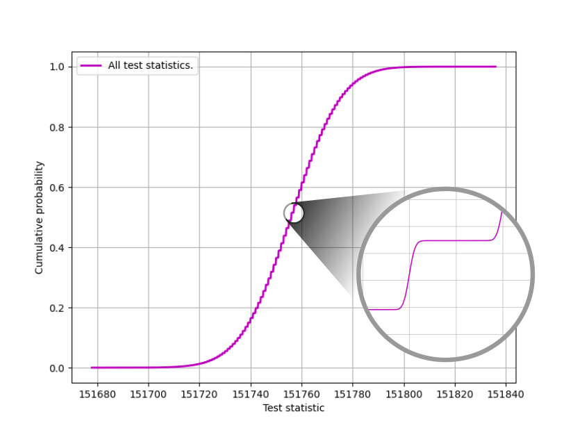
Raw training data for the 75,000 byte Compression test.
Notice the steps in the ‘curve’. This is due to discrete data and worsened by the fact that there are few categories, and so many repeats. But also note that the steps are not sharp and angular, but rather look like tinny normal distributions. That’s due to us adding $\mathcal{N}(0, 0.05^2)$ variates to the raw data during post processing. Thus the discrete distribution degenerates into indiscretion, or at least a continuous distribution if you will. It helps with downstream interpolation which does not fancy multiple identical $x$ values. There is no significant error introduced as the sum of a large number of normal variates is zero when $\mu = 0$. Sometimes though, the training curve might look like:-
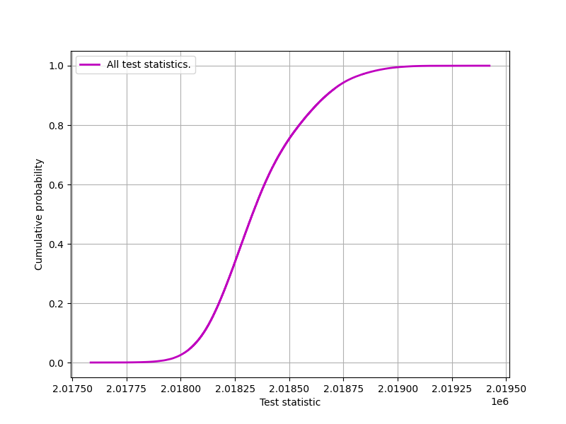
Raw training data for the 1,000,000 byte Compression test.
It’s markedly different. As are the eCDFs that arise within the Entropy test. Notice the differing spreads of $ts$ for various file sizes, indicating diminishing $\sigma$ as the samples file size increases:-
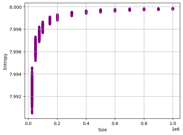
All raw training data for the Entropy test.
There is no algebraic technique to pre calculate these eCDFs (that we are aware of). This forms one of our justifications for using simulation.
Calibration encoding
The secret behind our simulation training.
We don’t really store all of the raw training data in the ent3000 test suite. We store the red dots in the chart below. They are 15 interpolated points after curve fitting.
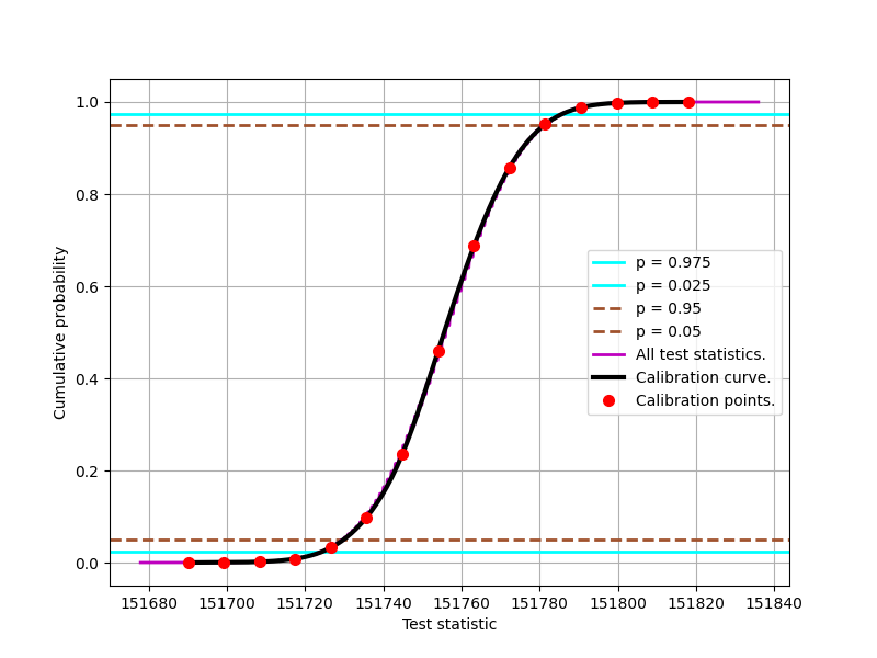
Calibration curve for the 75,000 byte Compression test.
Such calibration data looks like:-
[151690.07679305 151699.21621375 151708.35563445 151717.49505515
151726.63447584 151735.77389654 151744.91331724 151754.05273794
151763.19215864 151772.33157934 151781.47100003 151790.61042073
151799.74984143 151808.88926213 151818.02868283]
[2.00000000e-05 2.42321887e-04 1.66456500e-03 8.30700649e-03
3.25854352e-02 9.86538412e-02 2.35589378e-01 4.59842278e-01
6.87072013e-01 8.58230455e-01 9.51720895e-01 9.87973357e-01
9.97881724e-01 9.99762376e-01 9.99982000e-01]
This data is stored in the calibration.json file, which is not to be messed with! The empirical tests are inextricably tied to them.
How to determine an empirical p value?
Take for example the 75,000 byte Compression test. ent3000 will double compress the samples file, and that might result a test statistic of say 151,740 bytes. We offer that up to a curve interpolated from the appropriate calibration points, giving $p = 0.150$. In the case of the Compression test, we are only interested in how small the test statistic is, not how large. This is then a one sided test, and if $\alpha = 0.05$, $p > \alpha$ which is a “PASS”. The result would have been “FAIL” had $p$ been less than 0.05.
Some tests (to be added in the future) will be two sided with cut offs at $p = 0.025$ and $p=0.975$, such as the Darts test.