Individual test details
Entropy
Shannon entropy $(H)$ is the information density of the contents of the samples file, expressed as a number of bits per byte. For a general source, $X$ with $n$ categories of symbol:-
$$H(X) = ts = −\sum_{i=0}^n P(x_i) \log_2(P(x_i))$$
This test mirrors the old ent entropy test by featuring the same scan window of 8 bits. Unfortunately for reasons described in our rationale, we have no closed form solution to this. Instead we rely on simulation for the p value directly from the empirical cumulative distribution function (eCDF) for the test statistic $ts$.
You should expect $ts \approx $ 8 bits/byte.
Compression
Similarly to the entropy test above, no closed form determination of a p value is possible due to the overwhelming algorithmic complexity of the test. The test statistic is the size of the compressed samples file $S$, as:-
$$ ts = |LZMA(S)| + |BZ2(S)| $$
We rely on simulation for the p value directly from the eCDF for $ts$. We also believe that two attempts at compression are better than one. The LZMA and BZ2 compression algorithms are located in the xz-1.9.jar and commons-compress-1.21.jar libraries. These jar files should not be changed without consideration of re-calibrating the test’s embedded eCDF.
You should expect $ts$ to be slightly $> 2 \times |S|$.
Chi
The chi-square test $(\chi^2)$ is one of the most common tests for the randomness of data, and is extremely sensitive to errors.
The test’s approximation to the chi-squared distribution breaks down if expected frequencies are too low. It will normally be acceptable so long as no more than 20% of the categories have expected frequencies below 5. We surpass 5 by engineering the test to have an expected 34 counts per category (actually slightly greater). If we run the math $(\text{threshold} = 34 \times \text{bits} \times 2^{\text{bits}} /8)$, we arrive at the following minimum sample file lengths for bit windows of sizes 9 to 14. The larger the bit window, the more rigorous the test. ent uses a bit window of length 8.
| Bits | Categories | Threshold | Min.Length |
|---|---|---|---|
| 9 | 512 | 19,584 | 25,000 |
| 10 | 1,024 | 43,520 | 50,000 |
| 11 | 2,048 | 95,744 | 100,000 |
| 12 | 4,096 | 208,896 | 300,000 |
| 13 | 8,192 | 452,608 | 500,000 |
| 14 | 16,384 | 974,848 | 1,000,000 |
And finally the p value arises from the $\chi^2$ statistic using a standard Java library.
Mean
This is simply the result of summing all the bytes in the samples file and dividing by its length. If those bytes are random, the expectation should be 127.5. The variance of the mean is the sum of the variances, which for a discrete uniform distribution of single bytes is $\frac{256^2-1}{12}$. Thus for $n$ bytes:-
$$ \sigma^2 = \frac{256^2-1}{12n} = \frac{5,461.25}{n} $$
From here we calculate a standard Z score, $Z = \frac{ts - \mu}{\sigma},$ and finally a p value.
You should expect $ts \approx 127.5$.
Pi
To compute Monte Carlo estimates of $\pi$, we appropriate the function $f(x) = \sqrt(1 – x^2)$. The average function method is more accurate than ent’s area method because it has a smaller variance, thus is more rigorous. The graph of the function on the interval [0,1] is shown in the plot below. The curve forms a quarter circle of unit radius and the exact area under the curve is $\pi \over 4$.
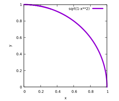
A quarter unit circle with area $\pi /4$.
We leverage the fact that the average value of a continuous function $f$ on the interval [a, b] is given by the following integral, $ f_{avg} = \frac{1}{b-a} \int_a^b f(x) dx $. That implies that for our curve:-
$$ f_{avg} = ts = \int_0^1 \sqrt(1 – x^2) dx = \frac{\pi}{4} $$
We convert four byte groups of the discrete sample distribution $S$ to normalised 32 bit reals as-
$$ \begin{align*} x = S_{3} &\ll 24 \vee \\ S_{2} &\ll 16 \vee \\ S_{1} &\ll 8 \vee \\ S_{0} &\ll 0 \\ \end{align*} $$
$$
x \leftarrow \frac{x}{2^{32} - 1}
$$
where the long denominator is $ 1111 \; 1111 \; 1111 \; 1111 \; 1111 \; 1111 \; 1111 \; 1111_2 $, $\ll n$ is an $n$ bit left shift and $\vee$ is logical OR. So after estimating the left hand side of the equation, we multiply the estimate by 4 to estimate $\pi$. And that’s its mean value, $ts$.
By magic and computing $E[(\sqrt{1-X^2})^2]=\int_0^1 (1-x^2) dx = 2/3$, so that now the variance of $\sqrt{1-X^2}$ is $E[1-X^2]-E[\sqrt{1-X^2}]^2=2/3-(\pi/4)^2,$ we determine that the variance of this estimate of $\pi$ is:-
$$ \sigma^2 = \frac{16}{n} \left\{ \frac{2}{3} - \left( \frac{\pi}{4} \right)^2 \right\} \approx \frac{0.797 \; 062 \; 266}{n} $$.
(Thanks to Ian for magical assistance with the variance formula.)
From here we calculate a standard Z score, $Z = \frac{ts - \mu}{\sigma}$, and finally a p value.
You should expect $ts \approx 3.141 \; 592 \; 653 $.
Uncorrelation
This quantity measures the extent to which each byte in the file depends upon the previous byte. We simply use a standard Java library to compute the Pearson’s correlation (R) between the original samples and another set of identical samples with a lag of 1.
The reasoning for calling this test Uncorrelation rather than Correlation as in the original ent is that ent displays the correlation coefficient, which is a test statistic $(ts)$. It’s not a p value. Our library returns a p value associated with the (two-sided) null hypothesis that the corresponding correlation coefficient is zero. Those are opposites, as in a good ent pass $ts \to 0$ whilst in a good ent3000 “PASS” $p \to 1$. Hence “Un…”
KS
Is a simple Kolmogorov–Smirnov test. We convert eight byte tuples of the discrete sample distribution $S$ to normalised 63 bit reals as-
$$ \begin{align*} x = (S_{7} \oplus 01111111_2) &\ll 56 \vee \\ S_{6} &\ll 48 \vee \\ S_{5} &\ll 40 \vee \\ S_{4} &\ll 32 \vee \\ S_{3} &\ll 24 \vee \\ S_{2} &\ll 16 \vee \\ S_{1} &\ll 8 \vee \\ S_{0} &\ll 0 \\ \end{align*} $$
$$
x \leftarrow \frac{x}{2^{63} - 1}
$$
where the long denominator is $ 0111 \; 1111 \; 1111 \; 1111 \; 1111 \; 1111 \; 1111 \; 1111 \; 1111 \; 1111 \; 1111 \; 1111 \; 1111 \; 1111 \; 1111 \; 1111_2 $, $\ll n$ is an $n$ bit left shift and $\vee$ is logical OR. We get 3,125 real data points for the smallest sample file size of 25,000 bytes. The standard Java library returns a p value directly when tested against $\mathcal{U}[0, 1]$.
Shells
This is fundamentally a $\chi^2$ test where the discrete sample distribution $S$ is floated to 24 bit x, y and z coordinates (apparently 72 bits of precision, see Double precision floating-point format) within a unit radius sphere looking like so:-
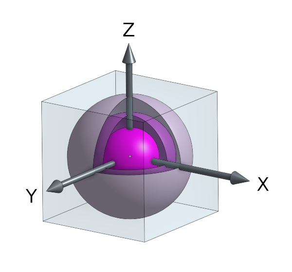
An example solid 3D sphere covered in thin shells.
We perform the same discrete to real byte transformation on $S$ as above, but this time only left shifting a maximum of 24 bits for each axis. We also create reals further mapped onto $\mathcal{U}[-1, 1]$ as for example $ x \leftarrow 2(x - 0.5) $ to fill the sphere’s enclosing cube of side 2. Then $r = \sqrt(x^2 + y^2 + z^2)$.
There is a solid core, enclosed by 99 thin shells. Magically the radii of the core and shells are such that all volumes are perfectly identical. This should result in roughly the same number of points within each, that can then be $\chi \text{’ed}$. Any points falling outside of the outer shell $(r > 1)$ are just ignored. 25,000 is the minimum sample size, thus most onerous.
This test is sensitive to the choice of bins. There is no optimal choice for the bin width (since the optimal bin width depends on the distribution). Most reasonable choices should produce similar, but not identical, results. For the chi-square approximation to be valid, the expected frequency should be at least 5. This test is not valid for small samples, and if some of the counts are less than five, you may need to combine some bins in the tails.
- NIST.
We’ve schemed to expect a minimum of 14 points /shell. Good enough. The magic radii are listed below, calculated from $r = \sqrt[3]{\frac{3V}{4 \pi}}$. The test is complementary to the KS test.
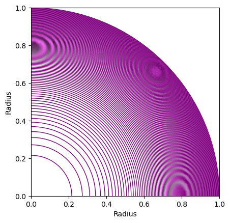
The core and all the shells, to scale.
And finally the p value arises from the $\chi^2$ statistic using a standard Java library.
Runs
The runs test can be used to decide if a data set is from a random process.
A run is defined as a series of increasing values or a series of decreasing values. The number of increasing $n_1$, or decreasing $n_0$, values is the length of the run. In a random data set, the probability that the (i+1)th value is larger or smaller than the ith value follows a binomial distribution, which forms the basis of the runs test.
The first step in the runs test is to count the number of runs in the data sequence. We will code values above the mean as “ones” and values below the median as “zeros”. A run is defined as a series of consecutive ones (or zero) values. The observed number of runs forms the test statistic ($ts$).
- NIST (With median cut off changed to mean by RRR).
The expected number of runs:-
$$ \mu = \frac{2 n_0 n_1}{n_0 + n_1} + 1 $$
and the standard deviation of the number of expected runs:-
$$
\sigma^2 =
\frac{2 n_0 n_1(2 n_0 n_1 - n_0 - n_1)} {(n_0 + n_1)^2 (n_0 + n_1 - 1)}
$$
From here we calculate a standard Normal Z score, $Z = \frac{ts - \mu}{\sigma}$, and finally a p value. We can make this Binomial to Normal approximation due to the large number of samples.